5. Transfer learning
Questions
How do I apply a pre-trained model to my data?
Objectives
Adapt a state-of-the-art pre-trained network to your own dataset
What is transfer learning?
Instead of training a model from scratch, with transfer learning you make use of models that are trained on another machine learning task. The pre-trained network captures generic knowledge during pre-training and will only be ‘fine-tuned’ to the specifics of your dataset.
An example: Let’s say that you want to train a model to classify images of different dog breeds. You could make use of a pre-trained network that learned how to classify images of dogs and cats. The pre-trained network will not know anything about different dog breeds, but it will have captured some general knowledge of, on a high-level, what dogs look like, and on a low-level all the different features (eyes, ears, paws, fur) that make up an image of a dog. Further training this model on your dog breed dataset is a much easier task than training from scratch, because the model can use the general knowledge captured in the pre-trained network.
        flowchart LR
    accTitle: Transfer Learning
    accDescr {The "Dogs & Cats" dataset is used to train a model.
    With Transfer Learning, the smaller "Dog Breeds" dataset is used to add more specific data.
    This results in the "Dog Breeds" model that makes use of both data sets.}
    A[(Dogs & Cats Data)] --> |Train Model| B(Model Dogs & Cats)
    C{Transfer Learning}
    B --> C
    D[(Dog Breeds Data)] --> C
    C --> E(Dog Breeds Model)
In this episode we will learn how to adapt a state-of-the-art pre-trained model to the Dollar Street Dataset.
1. Formulate / Outline the problem
Just like in the previous episode, we use the Dollar Street 10 dataset.
We load the data in the same way as the previous episode:
import pathlib
import numpy as np

DATA_FOLDER = pathlib.Path('data/dataset_dollarstreet/') # change to location where you stored the data
train_images = np.load(DATA_FOLDER / 'train_images.npy')
val_images = np.load(DATA_FOLDER / 'test_images.npy')
train_labels = np.load(DATA_FOLDER / 'train_labels.npy')
val_labels = np.load(DATA_FOLDER / 'test_labels.npy')
2. Identify inputs and outputs
As discussed in the previous episode, the input are images of dimension 64 x 64 pixels with 3 colour channels each. The goal is to predict one out of 10 classes to which the image belongs.
3. Prepare the data
Import the deep learning framework
Before we move on to the next section of the workflow we need to make sure we have Keras imported. We do this as follows:
from tensorflow import keras
import tensorflow as tf

keras.utils.set_random_seed(2)
Before we move on to the next section of the workflow we need to make sure we have PyTorch imported. We do this as follows:
import torch
import torchvision

torch.manual_seed(2)
We prepare the data as before, scaling the values between 0 and 1.
train_images = train_images / 255.0
val_images = val_images / 255.0
We introduce a dataset class here:
Similar as in the previous session: It scales the values between 0 and 1, but also permutes the order of dimensions as image data is organised differently in PyTorch than in tensorflow.
What is new is that, we introduce an callable attribute
transformto the dataset class. This function preprocesses the images before feeding them to our neural network. It is a good practice to do this in the dataset class as then the transformations are only executed for an image when fetching the image. In our lesson here it would be also fine to do these once, but in many cases one would then run out of memory.
class DollarStreetDataset(torch.utils.data.Dataset):
    def __init__(self, root, train=True, transform = None):
        prefix = "test"
        if train == True:
            prefix = "train"
        self.images = np.load(root / f'{prefix}_images.npy') / 255.
        self.labels = np.load(root / f'{prefix}_labels.npy')
        self.transform = transform

    def __getitem__(self, idx):
        # PyTorch requires another order of dimensions than the original tensorflow data
        x = torch.permute(torch.tensor(self.images[idx], dtype=torch.float), (2, 0, 1))

        # This is required as we would like to perform the transforms when fetching the data
        # Especially important, e.g., with large datasets or when doing augmentations
        if self.transform is not None:
            x = self.transform(x)
        y = torch.tensor(self.labels[idx], dtype=torch.long)
        return x, y

    def __len__(self):
        return self.images.shape[0]
4. Choose a pre-trained model or start building architecture from scratch
Note
In practice, you would probably first pick a pre-trained model, and then realise what pre-processing needs to be done. The steps below can be seen as the results of an iterative work.
Before loading any pre-trained model, we need to take care of the fact that our images have 64 x 64 pixels, whereas the pre-trained model that we will use was trained on images of 160 x 160 pixels.
Let’s define our model input layer using the shape of our training images:
# input tensor
inputs = keras.Input(train_images.shape[1:])
Our images are 64 x 64 pixels, whereas the pre-trained model that we will use was trained on images of 160 x 160 pixels. To adapt our data accordingly, we add an upscale layer that resizes the images to 160 x 160 pixels during training and prediction.
# upscale layer
method = tf.image.ResizeMethod.BILINEAR
upscale = keras.layers.Lambda(
  lambda x: tf.image.resize_with_pad(x, 160, 160, method=method))(inputs)
Our images are 64 x 64 pixels, whereas the pre-trained model that we will use was
trained on images of 160 x 160 pixels.
To adapt our data accordingly, we define a transform function that resizes the images to 160 x 160 pixels during training and prediction.
import torchvision.transforms as T

transform = T.Compose([
    T.ToPILImage(),
    T.Resize(160),        # keeps aspect ratio
    T.CenterCrop(160),    # ensures output is 160x160
    T.ToTensor()])
We pass our transform function when creating the train_dataset and val_dataset.
train_dataset = DollarStreetDataset(DATA_FOLDER, train=True, transform=transform)
val_dataset = DollarStreetDataset(DATA_FOLDER, train=False, transform=transform)
We use a DenseNet121. This architecture was proposed by the paper: Densely Connected Convolutional Networks (CVPR 2017). It is trained on the Imagenet dataset, which contains 14,197,122 annotated images according to the WordNet hierarchy with over 20,000 classes.
We will have a look at the architecture later, for now it is enough to know that it is a convolutional neural network with 121 layers that was designed to work well on image classification tasks.
From the keras.applications module we use the DenseNet121 architecture.
Let’s configure the DenseNet121:
base_model = keras.applications.DenseNet121(include_top=False,
                                            pooling='max',
                                            weights='imagenet',
                                            input_tensor=upscale,
                                            input_shape=(160,160,3),
                                            )
SSL: certificate verify failed error
If you get the following error message: certificate verify failed: unable to get local issuer certificate,
you can download the weights of the model manually
and then load in the weights from the downloaded file:
base_model = keras.applications.DenseNet121(
    include_top=False,
    pooling='max',
    weights='densenet121_weights_tf_dim_ordering_tf_kernels_notop.h5', # this should refer to the weights file you downloaded
    input_tensor=upscale,
    input_shape=(160,160,3),
)
By setting include_top to False we exclude the fully connected layer at the
top of the network, hence the final output layer. This layer was used to predict the Imagenet classes,
but will be of no use for our Dollar Street dataset.
Note that the ‘top layer’ appears at the bottom in the output of model.summary().
We add pooling='max' so that max pooling is applied to the output of the DenseNet121 network.
By setting weights='imagenet' we use the weights that resulted from training
this network on the Imagenet data.
We connect the network to the upscale layer that we defined before.
From the torchvision.models module we use the densenet121 architecture.
import torch.nn as nn

# We would like to specify a sensible path for this as this is where the pre-trained model is stored.
os.environ['TORCH_HOME']='.'

class DenseNetClassifier(nn.Module):
    def __init__(self, num_classes):
        super().__init__()

        # taking the pre-trained model from torchvision here, but throwing away the head
        self.backbone = nn.Sequential(
                            torchvision.models.densenet121(weights="IMAGENET1K_V1").features,
                            nn.AdaptiveMaxPool2d((1, 1)),
                            nn.Flatten())

        # creating our own head for classification
        self.head = nn.Sequential(nn.BatchNorm1d(1024),
                                        nn.Linear(1024, 50),
                                        nn.ReLU(),
                                        nn.Dropout(0.5),
                                        nn.Linear(50, num_classes))

    def forward(self, x):
        x = self.backbone(x)    # → [batch_dim, 1024]
        x = self.head(x)        # → [batch_dim, num_classes]
        return x
We would like to use only the feature extractor of the DenseNet and add our own classification head.
Thus, we use the torchvision.models.densenet121(weights="IMAGENET1K_V1").features subpart of the pre-trained DenseNet.
It maps each image to a vector of dimension 1024. The weights parameter here specifies that we use ImageNet as pre-training data.
Note that there are many different versions of ImageNet, but for this course it is fine that we use one version of ImageNet.
The self.head maps from the vector of dimension 1024 to a vector of dimension num_classes (10 in our case).
The choices here are arbitrary, one might as well as head only one layer of nn.Linear(1024, num_classes).
Only train a ‘head’ network
Instead of fine-tuning all the weights of the DenseNet121 network using our dataset, we choose to freeze all these weights and only train a so-called ‘head network’ that sits on top of the pre-trained network. You can see the DenseNet121 network as extracting a meaningful feature representation from our image. The head network will then be trained to decide on which of the 10 Dollar Street dataset classes the image belongs.
We will turn of the trainable property of the base model:
base_model.trainable = False
Let’s define our ‘head’ network:
out = base_model.output
out = keras.layers.Flatten()(out)
out = keras.layers.BatchNormalization()(out)
out = keras.layers.Dense(50, activation='relu')(out)
out = keras.layers.Dropout(0.5)(out)
out = keras.layers.Dense(10)(out)
Finally we define our model:
model = keras.models.Model(inputs=inputs, outputs=out)
In PyTorch, we can prevent updating layers of the model by setting the param.requires_grad property to False.
Here, we do that for the backbone part of the model as we would like to train the head.
model = DenseNetClassifier(num_classes=10)

for param in model.backbone.parameters():
    param.requires_grad = False
If you want to make sure, you could print all parameters of backbone and head and see if they are frozen or not.
print("Backbone parameters (should not be trainable)")
for name, param in list(model.backbone.named_parameters(prefix="backbone")):
    print(name, "trainable:", param.requires_grad)

print("\nBackbone parameters (should be trainable)")
for name, param in list(model.head.named_parameters(prefix="head")):
    print(name, "trainable:", param.requires_grad)
Inspect the DenseNet121 network
Have a look at the network architecture:
Use the following function:
model.summary()
Use the following lines to generate the summary:
from torchinfo import summary
summary(model, depth=2)
(We set the depth=2 to reduce the amount of lines printed.)
It is indeed a deep network, so expect a long summary!
1.Trainable parameters
How many parameters are there? How many of them are trainable?
Why is this and how does it effect the time it takes to train the model?
2. Head and base
Can you see in the model summary which part is the base network and which part is the head network?
3. Max pooling (relevant only for Keras)
Which layer is added because we provided pooling='max' as argument for DenseNet121()?
Solutions
1. Trainable parameters
Total number of parameters: 7,093,360, out of which only 53,808 are trainable.
The 53,808 trainable parameters are the weights of the head network. All other parameters are ‘frozen’ because we set base_model.trainable=False. Because only a small proportion of the parameters have to be updated at each training step, this will greatly speed up training time.
2. Head and base
The head network starts at the flatten layer, 5 layers before the final layer.
3. Max pooling (relevant only for Keras)
The max_pool layer right before the flatten layer is added because we provided pooling='max'.
1. Trainable parameters
Total number of parameters: 7,007,664, out of which only 53,808 are trainable.
The 53,808 trainable parameters are the weights of the head network. All other parameters are ‘frozen’ because we set param.requires_grad = False. Because only a small proportion of the parameters have to be updated at each training step, this will greatly speed up training time.
2. Head and base
The head network starts at the flatten layer, 5 layers before the final layer.
Training and evaluating the pre-trained model
Note that we have added more hints for PyTorch here as it requires more lines of code, but allows also for more customization.
1. Compile the model
Compile the model:
Use the
adamoptimizerUse the
SparseCategoricalCrossentropyloss withfrom_logits=True.Use ‘accuracy’ as a metric.
2. Train the model
Train the model on the training dataset:
Use a batch size of 32
Train for 30 epochs, but use an earlystopper with a patience of 5
Pass the validation dataset as validation data so we can monitor performance on the validation data during training
Store the result of training in a variable called
historyTraining can take a while, it is a much larger model than what we have seen so far.
3. Inspect the results
Plot the training history and evaluate the trained model. What do you think of the results?
4. (Optional) Try out other pre-trained neural networks
Train and evaluate another pre-trained model from keras applications. How does it compare to DenseNet121?
1. Define training and test loops
We first define two functions similar to session 4 that train and test the model.
from tqdm import tqdm

def train(dataloader, model, loss_fn, optimizer, device):
    model.train()
    train_loss = 0
    correct = 0
    total = 0

    # this tdqm magic is only there to make this progress bar appear
    for step, (x, y) in (enumerate(pbar:=tqdm(dataloader))):
        x, y = x.to(device), y.to(device)
        optimizer.zero_grad()
        logits = model(x)
        loss = loss_fn(logits, y)
        loss.backward()
        optimizer.step()
        train_loss += loss.item() * x.size(0)
        preds = logits.argmax(dim=1)
        correct += (preds == y).sum().item()
        total += y.size(0)
        pbar.set_description(f"Loss: {(loss.item()):>7f}")

    train_loss /= total
    train_acc = correct / total


    return train_loss, train_acc

def test(dataloder, model, loss_fn, device=torch.device("cuda:0")):
    model.eval()
    val_loss = 0
    correct = 0
    total = 0
    with torch.no_grad():
        for x, y in dataloder:
            x, y = x.to(device), y.to(device)
            logits = model(x)
            loss = loss_fn(logits, y)
            val_loss += loss.item() * x.size(0)
            preds = logits.argmax(dim=1)
            correct += (preds == y).sum().item()
            total += y.size(0)

        val_loss /= total
        val_acc = correct / total

    return val_loss, val_acc
2. Train the model
We use our train and test functions together with other objects know from prior sessions.
Note that in PyTorch early stopping needs to be defined by you as there is no predefined class as in Keras.
from torch.utils.data import DataLoader
from torch.optim import Adam


# take a GPU as default when it is available
device = "cuda" if torch.cuda.is_available() else "cpu"


model = model.to(device)
optimizer = Adam(model.parameters(), lr=0.001) # learning rate is here set to the same as in Keras default
loss_fn = nn.CrossEntropyLoss()

train_loader = DataLoader(train_dataset, batch_size=32, shuffle=True)
val_loader = DataLoader(val_dataset, batch_size=32)

num_epochs = 30

# for early stopping
best_val_loss = float("inf")
patience = 5
wait = 0

# for bookkeeping
history = {"epoch": [], "train_loss": [],    "train_acc": [],    "val_loss": [],    "val_acc": []}

for epoch in range(num_epochs):
    train_loss, train_acc = train(dataloader=train_loader, model=model, loss_fn=loss_fn, optimizer=optimizer, device=device)
    val_loss, val_acc = test(dataloder=val_loader, model=model, loss_fn=loss_fn, device=device)


    # Save to history
    history["epoch"].append(str(epoch+1))
    history["train_loss"].append(train_loss)
    history["train_acc"].append(train_acc)
    history["val_loss"].append(val_loss)
    history["val_acc"].append(val_acc)


    # print progress
    print(f"Epoch {epoch+1}/{num_epochs} ",
    f"Train Loss: {train_loss:.4f} Train Acc: {train_acc:.4f} ",
    f"Val Loss: {val_loss:.4f} Val Acc: {val_acc:.4f}")

    # Early stopping (there is not a build-in version for that in PyTorch)
    if val_loss < best_val_loss:
        best_val_loss = val_loss
        wait = 0
        torch.save(model.state_dict(), "best_model.pt")
    else:
        wait += 1
        if wait >= patience:
            print("Early stopping triggered.")
            break

print(f"Training complete at epoch {epoch+1}")
3. Inspect the results
You can plot the results yourself or have a look at the plotting in the solution.
4. (Optional) Try out other pre-trained neural networks
Train and evaluate another pre-trained model from torch vision. How does it compare to DenseNet121?
Solution
1. Compile the model
model.compile(optimizer='adam',
              loss=keras.losses.SparseCategoricalCrossentropy(from_logits=True),
              metrics=['accuracy'])
2. Train the model
Define the early stopper:
early_stopper = keras.callbacks.EarlyStopping(monitor='val_accuracy',
                              patience=5)
Train the model:
history = model.fit(x=train_images,
                    y=train_labels,
                    batch_size=32,
                    epochs=30,
                    callbacks=[early_stopper],
                    validation_data=(val_images, val_labels))
3. Inspect the results
def plot_history(history, metrics):
    """
    Plot the training history

    Args:
        history (keras History object that is returned by model.fit())
        metrics(str, list): Metric or a list of metrics to plot
    """
    history_df = pd.DataFrame.from_dict(history.history)
    sns.lineplot(data=history_df[metrics])
    plt.xlabel("epochs")
    plt.ylabel("metric")

plot_history(history, ['accuracy', 'val_accuracy'])
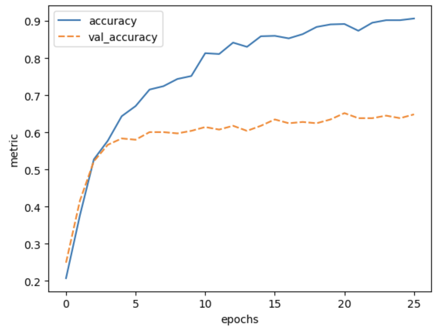 The final validation accuracy reaches 64%, this is a huge improvement over 30% accuracy we reached with the simple convolutional neural network that we build from scratch in the previous episode.
1. See solution in exercise
2. See solution in exercise
3. Inspect the results
def plot_history(history, metrics):
    history_df = pd.DataFrame.from_dict(history)
    for metric in metrics:
        sns.lineplot(data=history_df, x="epoch",y=metric, label=metric, marker="o")
    plt.xlabel("epochs")
    plt.ylabel("metric")

plot_history(history, ['train_acc', 'val_acc'])
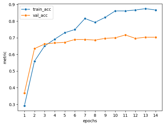 The final validation accuracy reaches 64%, this is a huge improvement over the accuracy we reached with the simple convolutional neural network that we build from scratch in the previous episode.
Concluding: The power of transfer learning
In many domains, large networks are available that have been trained on vast amounts of data, such as in computer vision and natural language processing. Using transfer learning, you can benefit from the knowledge that was captured from another machine learning task. In many fields, transfer learning will outperform models trained from scratch, especially if your dataset is small or of poor quality.
Transfer learning adapts a model to a specific dataset. This typically leads to improvements in the particular domain covered by the data. Research has shown, however, that fine-tuning the model weights like this can have negative side effects on the model performance in other domains so that a specialized, fine-tuned model must be re-evaluated before using it for more generic tasks.
Keypoints
Large pre-trained models capture generic knowledge about a domain
Use the
keras.applicationsortorchvision.modelsmodule to easily use pre-trained models for your own datasetsAs usual with all options, there can be drawbacks to using pre-trained models.